Cyrus Samii

Tracy L. Nolen and Michael G. Hudgens have new paper posted to JASA’s preprint website (gated link, ungated preprint) on randomization inference in situations where intermediate post-treatment outcomes are important in defining causal effects. Their motivating example is one where we want to see how a medical treatment affects people’s recovery from an infection, but infection status is something that is itself affected by the treatment. Other examples where post-treatment outcomes are important are estimating causal effects under noncompliance and related instrumental variables methods (classic paper link), as well as the “truncation by death” situation (link) for which causal effects are only meaningful for certain endogenously revealed subpopulations. In these cases, principal strata refer to subpopulations that are distinguished by intermediate potential outcomes. The key contribution here is to develop exact tests for principal strata estimation. The authors want to use exact tests, rather than asymptotic-frequentist or Bayesian approaches, because exact tests have better type-I/type-II error performance in small samples, and many principal strata situations involve making inferences on small subgroups of, possible already-small, subject pools.

To formalize their argument a bit, let $latex Z_i =0,1$ refer to a subject’s treatment status, $latex S_i =0,1$ refer to a subject’s infection status (observed after treatment), and $latex y_i(S_i|Z_i)$ refer to a subject’s outcome given infection and treatment statuses. We are interested in the effect of treatment on progress after infection:

$latex E[y_i(S=1|Z=1) – y_i(S=1|Z=0)]$.

(Clearly this estimand is only meaningful for those that could be infected under either condition.) But,

$latex E[y_i(S_i=1|Z_i=1)] \ne E[y_j(S_j=1|Z_j=1)]$

and

$latex E[y_i(S_i=1|Z_i=0)] \ne E[y_j(S_j=1|Z_j=0)]$

for $latex i$ in treated and $latex j$ in control, because $latex S$ is endogenous to $latex Z$. Thus, the expression,

$latex E[y_i(S_i=1|Z_i=1)] – E[y_j(S_j=1|Z_j=0)]$

for $latex i$ in treated and $latex j$ in control does not estimate the effect of interest. In terms of principal strata, $latex y_i(S_i=1|Z_i=1)$ is an element in a sample from the mixed population of people for whom $latex S=1$ only when $latex Z=1$ (the “harmed” principal stratum) or $latex S=1$ irrespective of $latex Z$ (the “always infected” principal stratum), while $latex y_j(S_j=1|Z_j=0)$ is an element in a sample from the mixed population of people for whom $latex S=1$ only when $latex Z=0$ (“protected”) or $latex S=1$ irrespective of $latex Z$ (“always infected”). The two mixed populations are thus different and it is reasonable to expect that treatment effects also differ across these two subpopulations. For example, imagine that “the harmed” are allergic to the treatment but otherwise very healthy, and so the treatment not only causes the infection but leads to an allergic reaction that catastrophically interferes with their bodies’ responses to infection. In contrast, suppose the “protected” are in poor health; their infection status may respond to treatment, but their general prognosis is unaffected and is always bad. Finally, suppose the “always infected” do not respond to treatment in their outcomes either. Here, on average, the treatment is detrimental due to the allergic response among “the harmed”. But if one estimates a treatment effect by comparing these two subpopulations, one may find that the treatment is on average benign. This is a made-up example, but does not seem so far-fetched at all. [Update: Upon further reflection, I realize that the preceding illustration that appeared in the original post had a problem: it failed to appreciate that the causal effect of interest here is only properly defined for members of the “always infected” population. The point about bias still holds, but it arises because one is not simply taking difference in means between treated and control “always infected” groups, but rather between the two mixed groups described above. The problem, then, is to find a way to isolate the comparison between treated and control “always infected” groups, removing the taint introduced from the presence of the “harmed” subgroup among the treated and the “protected” subgroup among the control. This is interesting, because it is precisely the opposite of what one would want to isolate in a LATE IV analysis. Nonetheless, the identifying condition is the same — as discussed below, it hinges on monotonicity.]

The authors construct an exact test for the null hypothesis of no treatment effect within a given principal stratum under a monotonicity assumption that states that the treatment can only affect infection status in one direction (essentially, this is the same “no defier” monotonicity assumption that Angrist, Imbens, and Rubin use to identify the LATE IV estimator). This rules out the possibility of anyone being in the “harmed” group. The assumption thus allows you to bound the number of people in each of the remaining principal strata (“always infected”, “protected”, and “never infected”). Then, an exact test can be carried out that computes the maximum exact test p-value under all principal stratum assignments consistent with these bounds. The analysis can assess consequences of violations of monotonicity through a sensitivity analysis: the proportion of “harmed” can be fixed by the analysts and the test re-computed to assess robustness.

An alternative approach used in the current literature is what is called the “burden of illness” approach (BOI). BOI collapses intermediate and endpoint outcomes into a single index and then carries out an ITT analysis on this index. The authors find that their exact test on principal strata has substantially more power than BOI ITT analysis. The authors also show that Rosenbaum (2002) style covariate adjustment can be applied (regress outcomes on covariates, perform exact test with residuals), and the usual inverted exact test confidence intervals can be used, both with no added complication.

It’s a nice paper, related to some work that some colleagues and I are currently doing on randomization inference. Exact tests are fine for null hypothesis testing, but I am not at all sold on constant-effects-based inverted exact tests for confidence intervals. Certainly for moderate or large samples, there is no reason at all to use such tests, which can miss the mark badly. Maybe for small samples though you don’t really have a choice.

My co-researchers and I are currently analyzing data that we have collected as part of the Nepal Peacebuilding Survey, a multipurpose survey in 96 hamlets across Nepal studying the impact of wartime violence with implications for peacebuilding policy. Some background is here (link). Our implementation partner is New Era Nepal (link).

To inform our analysis, I’ve conducted a review of findings from qualitative (that is, ethnographic and journalistic) accounts of the effects of wartime violence in rural areas. I’m posting the review here (PDF) as a reference for others who might be interested. It is written in a very succinct style, and it presumes a good amount of previous knowledge about the 1996-2006 conflict between Maoist and state forces. Good background information is available on the web from, e.g., the International Crisis Group (link).

Comments are very welcome, either here in the comments section or via email. I’m especially interested in recommendations of additional literature or comments explaining different interpretations of the findings in this literature. I’ll share more on the findings from the data analysis as we complete it.

With the Cote d’Ivoire election crisis having moved toward resolution, there is a lot of discussion about how to deal with the challenges posed by close, contested elections. For example, Knox Chitiyo provides a great analysis in a BBC report (link), emphasizing the need for creating “higher, independent judicial” bodies “to resolve post-electoral disputes”, and noting how international support for Ouattara in Cote d’Ivoire suggests a turn away from “the power-sharing default setting” that informed the approach to the recent election crises in Kenya (2008) and Zimbabwe (2008-9). Now is the time to think about a whole range of measures that can be used to minimize uncertainty about the validity of vote counts, and commit candidates to accepting validated results.

I thought I’d look at some data to help put the recent Cote d’Ivoire crisis into context. Conveniently enough, Staffan Lindberg at the University of Florida has provided a freely available African elections dataset covering 1969-2007 (link). The graphics posted below display some trends, using only data since 1980 (the pre-1980 data is quite patchy).

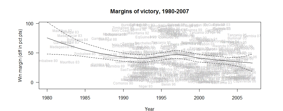
Figure 1 shows that close elections are increasingly the norm in Africa. The figure shows margins of victory for executive offices in both presidential and parliamentary elections since 1980. A trend line with error margins is overlaid (based on a loess fit). Whereas prior to 1990, landslides were the norm, since then close elections have become increasingly common. Interestingly, in very recent years, we see that there cease to be any “near 100%” margin-of-victory elections. This may reflect the effects of increased citizen awareness and activism, given that such outcomes are incompatible with free-and-fair elections process when there is any modicum of pluralism.

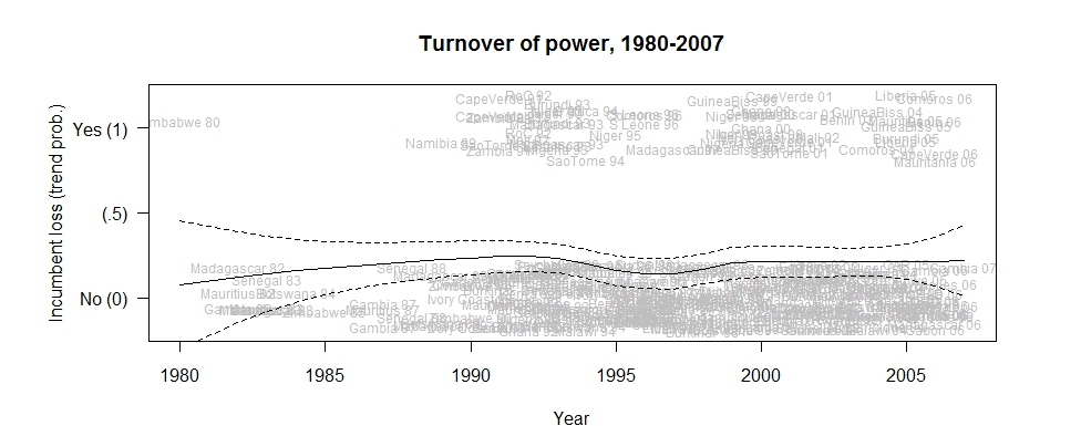
Figure 2 shows the flip side of the same coin, displaying trends in executive incumbent losses and resulting turnover since 1980. Consistent with what Figure 1 shows in terms of margins of victory, elections have become more competitive, with the proportion of elections resulting in executive turnover having risen from almost zero to about 25% as of 2007.

Figure 3 looks at how margins of victory and incumbent losses relate. In a free and fair system, there should be a systematic relationship between the two. Namely, a margin of victory of about 0 suggests a tie between the two front-runners. In such cases, assuming that the two front-runners have equal resources, it should be that each front runner has about a 50% chance of winning. In nearly all of the elections in these data, one of the front-runners is an incumbent or incumbent-party candidate. Thus, in close elections, we should see about a 50-50 split in whether or not there is an incumbent loss and consequent turnover of executive power.

Figure 3 shows that overall since 1980, this has not quite been the case, as incumbents and incumbent parties have lost only 40% of the time. However, when we break this out over time, we see that the pattern is converging to the expected outcome in fair elections. In 1980-1990, margins of victory were never close to zero, and so this phenomenon was unobservable. In 1990-2000, we see that there were many close elections, but that the outcomes were dominated by incumbents. Notice that with the exception of Niger 1993, those clumped very close to zero are almost entirely incumbent victories. This is suggestive of some electoral shenanigans. A possible story is that some portion of these elections were due to be incumbent losses, but that some form of fraud was perpetrated by incumbents (who, after all, are in a position of strength to do so) to ensure that the loss did not occur. This is just a conjecture, though. Note that such signs of incumbent advantage in close elections are not unique to Africa. For some US examples, see this past post (link).

But as the third graph in Figure 3 shows, in the past decade, the pattern expected of fair elections is evident. The predicted probability of an incumbent loss when the margin of victory is zero is 0.48, which is almost exactly the 0.50 that one would expect.

Although these data are too coarse to really allow us to tell what is going on, it does provide some reason for optimism about the effects of increased citizen awareness, increased opposition capacity building, and more benevolent international assistance in improving electoral outcomes in Africa.

Figure 1: Trends in margins of victory

Figure 2: Trends in incumbent losses and resulting executive turnover

Figure 3: Margins of victory and likelihood of incumbent turnover

Here (link) is a note working through some algebra for comparing the following:

1. The Neyman “conservative” estimator for the variance of the difference-in-means estimator for the average treatment effect. This estimator is derived by applying sampling theory to the case of a randomized experiment on a fixed population or sample. Hardcore experimentalists might insist on using this estimator to derive the standard errors of a treatment effect estimate from a randomized experiment. This is also known as the conservative “randomization inference” based variance estimator.
   
   
2. The Huber-White heteroskedasticity robust variance estimator for the coefficient from a regression of an outcome on a binary treatment variable. This is a standard-use estimator for obtaining standard errors in contemporary econometrics. Taking from Freedman’s famous words, though, “randomization does not justify” this estimator.

If you work through the algebra some more, you will see that they are equivalent in balanced experiments, but not quite equivalent otherwise.

This post is part of a series of little explorations I’ve been doing into variance estimators for treatment effects. See also here, here, and here.

UPDATE 1 (4/8/11): A friend notes also that under a balanced design, the homoskedastic OLS variance estimator is also algebraically equivalent. When the design is not balanced, the homoskedastic and heteroskedastic robust estimators can differ quite a bit, with the latter being closer to the Neyman estimator, but still not equivalent to the Neyman estimator due to the manner in which treated versus control group residuals are weighted.

UPDATE 2 (4/12/11): The attached note is updated to carry through the algebra showing that the difference between the two estimators is very slight.

UPDATE 3 (4/12/11): A reader pointed out via email that this version of the heteroskedasticity robust estimator is known as “HC1”, and that Angrist and Pischke (2009) have a discussion of alternative forms (see Ch. 8, especially p. 304). From Angrist and Pischke’s presentation, we see that HC2 is exactly equivalent to the Neyman conservative estimator, and this estimator is indeed available in, e.g., Stata.

UPDATE 4 (4/12/11): Another colleague pointed out (don’t you love these offline comments?) that the Neyman conservative estimator typically carries an N/(N-1) finite sample correction premultiplying the expression shown in the note, in which case even in a balanced design, the estimators differ on the order of 1/(N-1). Later discovered that this was not true.

In the advance access pages of the American Journal of Epidemiology, Jonathan M. Snowden, Sherri Rose, and Kathleen M. Mortimer have a nice tutorial on what they refer to as “G-computation” for causal inference with observational data (ungated link). An average causal effect for a binary treatment can be defined as the average of individual level differences between the outcome that obtains when one is in treatment versus in control. Because people are either in treatment or control, one of these two “potential” outcomes is unobserved, or missing (within subjects designs do not overcome this, because the ordering of treatment assignment is itself another dimension of treatment). Given this “missing data” problem, G-computation refers to fitting models to available data that allow you to impute (i.e., predict) unobserved counterfactual values. You can then use this complete set of counterfactual values to estimate various types of causal effects. The idea isn’t so new or groundbreaking, but many theoretical insights have been elucidated only recently. Snowden et al’s presentation focuses on effects that average over the entire population.

These authors don’t cite it in their paper, but I think the most sophisticated application of this approach for a cross-sectional study is Jennifer Hill’s “Bayesian Nonparametric Modeling for Causal Inference” study (gated link). Hill uses the magical BART algorithm to fit a response surface and generate the imputations, from which various flavors of causal effect might be constructed (okay, full disclosure—Hill was one of my grad school teachers, but hey, BART is pretty cool). I understand that there has been a fair amount of application, at least beta-testing, of such counter-factual imputation methods in longitudinal studies as well, although I don’t have references handy.

This approach is especially appealing when you anticipate lots of measurable effect modification that you want to average-over in order to get average treatment effects. Actually, I think Snowden et al’s article does a good job of demonstrating how in some cases, it’s not classic confounding and omitted variable bias per se that is the major concern, but rather effect modification and effect heterogeneity (i.e., interaction effects) associated with variables that also affect treatment assignment. Traditional regression is clumsy in dealing with that. As far as I know conventional social science teaching, rooted as it is in constant effects models, does not have a catchy name for this kind of bias; maybe we can call it “heterogeneity bias.” Another thing that makes this kind of bias special relative to the usual kinds of confounding is that, as far as I understand, imputation-based strategies (like g-computation) that try to correct for it may in fact take advantage of measured heterogeneity associated with post-treatment variables. That is one of the reasons that these methods have appeal for longitudinal studies. (On this point, I’ll refer you to a little tutorial that I’ve written on a related set of methods—augmented inverse propensity weighting for attrition and missing data problems (link).)

Stijn Vansteelandt and Niels Keiding provide an invited commentary (gated link) on Snowden et al’s paper, and they make some really interesting points that I wanted to highlight. First, they note that imputation based strategies such as g-computation have a long history in association with the concept of “standardization.” More importantly are two points that they make later in their commentary. First is a point that Vansteelandt has made elsewhere, discussing the similarities and differences between imputation/standardization and inverse probability weighting:

The IPTW [inverse probability of treatment] approach is not commonly used in practice because of the traditional reliance on out- come-regression-based analyses, which tend to give more precise estimates. Its main virtue comes when the con- founder distribution is very different for the exposed and unexposed subjects (i.e., when there is near violation of the assumption of the experimental treatment assignment), for then the predictions made by the G-computation approach may be prone to extrapolate the association between out- come and confounders from exposed to unexposed subjects, and vice versa. The ensuing extrapolation uncer- tainty is typically not reflected in confidence intervals for model-based standardized effect measures based on tradi- tional outcome regression models, and thus the IPTW approach may give a more honest reflection of the overall uncertainty (provided that the uncertainty resulting from estimation of the weights is acknowledged) (19). A further advantage of the IPTW approach is that it does not re- quire modeling exposure effect modification by covariates and may thus ensure a valid analysis, even when effect modification is ignored.

I think this is an exceptionally important point, making clear that the apparent “inefficiency” of IP(T)W relative to imputation based methods is, in some sense, illusory. Vansteelandt and Keiding also discuss one approach to combining imputation and IPW in order to get the best of both worlds:

We here propose a compromise that combines the benefits of G-computation/ model-based standardization and of the IPTW approach. Its implementation is not more difficult than the implementa- tion of these other approaches. As in the IPTW approach, the first step involves fitting a model of the exposure on relevant covariates; this would typically be a logistic re- gression model. The fitted values from this model express the probability of being exposed and are commonly called ‘‘propensity scores.’’ They are used to construct a weight for each subject, which is 1 divided by the propensity score if the subject is exposed and 1 divided by 1 minus the pro- pensity score if the subject is unexposed. The second step involves fitting a model, the Q-model, for the outcome on the exposure and relevant covariates but using the afore- mentioned weights in the fitting procedure (e.g., using weighted least squares regression). Once estimated, the implementation detailed in the article by Snowden et al. (4) is followed; that is, counterfactual outcomes are pre- dicted for each observation under each exposure regimen by plugging a 1 and then subsequently a 0 into the fitted regression model to obtain predicted counterfactual outcomes. Finally, differences (or ratios) between the aver- age predicted counterfactual outcomes corresponding to different exposure regimens are calculated to arrive at a stan- dardized mean difference (or ratio) (see reference 19 for a similar implementation in the context of attributable fractions). We refer to this compromise approach as doubly robust standardization. Here, the name doubly robust expresses that doubly robust standardized effect measures have 2 ways to give the right answer: when either the Q-model or the propensity score model is correctly specified, but not necessarily both.

This approach has been demonstrated elsewhere—e.g. a recent paper by Vansteelandt and co-authors in the journal Methodology (ungated version, gated published). I am intrigued by this because it differs from the manner in which I have implemented doubly robust estimators that combine weighting and imputation (again, see link). I wonder if there is a difference in practice.