Cyrus Samii

At the Yale field experiments workshop today, Katherine Casey from Brown University (soon to be Stanford GSB) presented a brilliantly executed study by herself, Rachel Glennerster, and Edward Miguel evaluating the impact of a community directed development (CDD) program on local public goods and community social institutions in rural Sierra Leone. Here is a link to the working paper (PDF). I think this paper is a must-read for those interested not only in decentralization and democratization of rural social institutions in poor countries, but in field experiments, policy analysis, and causal inference more generally. In fact, I would suggest that if you have an interest in any of these things, that you stop what you are doing (including reading this post) and look carefully at their paper right now. Here is the abstract,

Although institutions are believed to be key determinants of economic performance, there is limited evidence on how they can be successfully reformed. The most popular strategy to improve local institutions in developing countries is “community driven development” (CDD). This paper estimates the impact of a CDD program in post-war Sierra Leone using a randomized experiment and novel outcome measures. We find positive short-run effects on local public goods provision, but no sustained impacts on fund-raising, decision-making processes, or the involvement of marginalized groups (like women) in local affairs, indicating that CDD was ineffective at durably reshaping local institutions.

They indicate that, for the most part, these results are consistent with what other CDD studies have produced, raising serious questions about donors’ presumptions that CDD programs can really affect local social institutions. In a recent review of CDD impact evaluations, my co-authors and I found the same thing (see here, gated link). Given the centrality of CDD programs in current development programming, this comes as a call to reflect a bit on why things might not be going as we would like.

For those who don’t really care that much about CDD, there are four methodological aspects of this paper that are simply terrific and therefore warrant that you read it:

1. They very effectively address the multiple outcomes, multiple comparisons, and associated “data dredging” problems that have plagued research on CDD in particular (see again our review essay) and pretty much every recent analysis of a field experiment that I have read. Their approach involves a few steps, with the last step being the most innovative. The steps are, first, articulating a clear set of core hypotheses and registering (via a Poverty Action Lab evaluation registry) these before the onset of the program; second, grouping outcome indicators as the bases of tests for these hypotheses; third, pre-specifying and registering their econometric models; and, finally, using seemingly-unrelated regressions (SUR, link) to produce standard errors on individual outcomes while taking into account dependence across indicators, and then using omnibus mean-effects tests to obtain a single standardized effect and p-value for each core hypothesis. For example, to test the hypothesis that the program would increase lasting social capital, they have about 40 measures. The SUR produces dependence-adjusted standard errors on each of these outcomes, and then the omnibus mean-effects test allows them to combine the results from these individual regressions to present a single standardized effect and p-value for the social capital hypothesis. That’s a huge step forward for analyses of field experiments. Effect synthesis and omnibus testing like this needs to become much more regularized in our statistical practice (see here for a recent post on omnibus tests of covariate balance).
   
   
2. Their hypotheses are motivated by a clear theoretical model that formalizes what the authors understand as being donors’ and the Bank’s thinking about how CDD affects community-level social dynamics. The model explains what constraints and costs they hypothesize as being alleviated such that the program might improve public goods and, potentially, social capital outcomes. This really shores up one’s confidence in the results of the empirical analysis, because it is clear how the hypotheses were ex ante established prior to the analysis.
   
   
3. A propos to some recent discussion over at the World Bank Development Impact blog (link), they study outcomes measured both during the program cycle and some time afterward, to assess programmatic effects on provision of public goods and downstream effects on social capital.
   
   
4. To measure effects on social capital, they created minimally intrusive performance measures based on “structured group activities” that closely resemble real-world situations in which collective problem solving would be required. For example, a social capital measure was based on the offer of a matching grant to communities, with the only condition to receive the grant being that the community had to coordinate to come up with matching funds and put-in for the grant. In the event, they found that only about half of communities overall were able to take up the matching grant, and the treatment effect on this take-up rate was effectively zero.

Katherine indicated that for them, the null result on social capital effects was the most important take-away point. This provoked a salient question during the Q&A: how will journal editors react to this, that the core finding of the paper is a null result on a hypothesis that was derived from a theory that was motivated only because it seemed to characterize what donors and Bank program staff thought would happen? As a political scientist, I am sympathetic to this concern. I can imagine the cranky political science journal editor saying, “Aw, well, this was a stupid theory anyway. Why should I publish a null result on an ill-conceived hypothesis? Why aren’t they testing a better theory that actually explains what’s going on? I mean, why don’t they use to data to prove the point that they want to make and teach us what is really going on?” Reactions like this, which I do hear fairly often, come in direct tension with ex ante science, and essentially beg researchers to do post-hoc analysis. Hopefully publishing norms in economics won’t force the authors to spoil what is a great paper and probably the most well-packaged, insightful null result I’ve ever read.

In their 2008 Statistical Science article, Hansen and Bowers (link) propose randomization-based omnibus tests for covariate balance in randomized and observational studies. The omnibus tests allow you to test formally whether differences across all the covariates resemble what might happen in a randomized experiment. Previous to their paper, most researchers tested balance one covariate at a time, making ad hoc judgments about whether apparent imbalance in one or another covariate suggested deviations from randomization. What’s nice about Hansen and Bowers’s approach is that it systematizes such judgments into a single test.

To get the gist of their approach, imagine a simple random experiment on $latex N$ units for which $latex M = N/2$ [CDS: note, this was corrected from the original; results in this post are for a balanced design, although the Hansen and Bowers paper considers arbitrary designs.] units are assigned to treatment. Suppose for each unit i we record prior to treatment a $latex P$-dimensional covariate, $latex x_i = (x_{i1},\hdots,x_{iP})’$. Let $latex \mathbf{X}$ refer to the $latex N$ by $latex P$ matrix of covariates for all units. Define $latex d_p$ as the difference in the mean values of covariate $latex x_p$ for the treated and control groups, and let $latex \mathbf{d}$ refer to the vector of these differences in means. By random assignment, $latex E(d_p)=0$ for all $latex p=1,..,P$, and $latex Cov(\mathbf{d}) = (N/(M^2))S(\mathbf{X})$, where $latex S(\mathbf{X})$ is the usual sample covariance matrix [CDS: see update below on the unbalanced case]. Then, we can compute the statistic, $latex d^2 = \mathbf{d}’Cov(\mathbf{d})^{-1} \mathbf{d}$. In large samples, Hansen and Bowers explain that randomization implies that this statistic will be approximately chi-square distributed with degrees of freedom equal to $latex rank[Cov(\mathbf{d})]$ (Hansen and Bowers 2008, 229). The proof relies on standard sampling theory results.

These results from the setting of a simple randomized experiment allow us to define a test for covariate balance in cases where the data are not from an experiment, but rather from a matched observational study, or where the data were from an experiment, but we might worry that there were departures from randomization that lead to confounding. In Hansen and Bowers’s paper, the test that they define relies on the large sample properties of $latex d^2$. Thus, the test consists of computing $latex d^2$ for the sample at hand, and computing a p-value against the limiting $latex \chi^2_{rank[Cov(\mathbf{d})]}$ distribution that should obtain under random assignment.

I should note that in Hansen and Bowers’s paper, they focus not on the case of a simple randomized experiment, but rather on cluster- and block-randomized experiments. It makes the math a bit uglier, but the essence is the same.

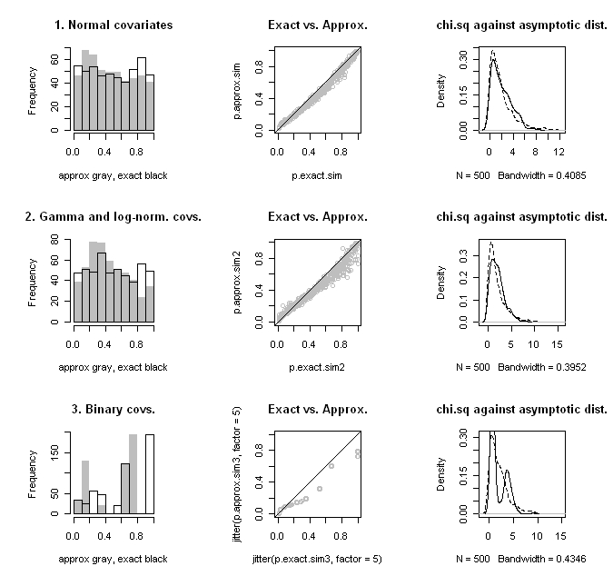
The question I had was, what is the small sample performance of this test? In small samples we can use $latex d^2$ to define an exact test. Does it make more sense to use the exact test? In order to address these questions, I performed some simulations against data that were more or less behaved. These included simulations with two normal covariates, one gamma and one log-normal covariate, and two binary covariates. (For the binary covariates case, I couldn’t use a binomial distribution, since this sometimes led to cases with all 0’s or 1’s. Thus, I fixed the number of 0’s and 1’s for each covariate and randomly scrambled them over simulations.) In the simulations, the total number of units was 10, and half were randomly assigned to treatment. Note that this implies 252 different possible treatment profiles.

The results of the simulations are shown in the figure below. The top row is the for the normal covariates, the second row for the gamma and log-normal covariates, and the bottom row for the binary covariates. I’ve graphed the histograms for the approximate and exact p-values in the left column; we want to see a uniform distribution. In the middle column is a scatter plot of the two p-values with a reference 45-degree line; we want to see them line up on the 45-degree line. In the right column, I’ve plotted distribution of the computed $latex d^2$ statistic against the limiting $latex \chi^2_{rank[Cov(\mathbf{d})]}$ distribution; we want to see that they agree.

When the data are normal, the approximation is quite good, even with only 10 units. In the two latter cases, approximations do not fare well, as the test statistic distribution deviates substantially from what would be expected asymptotically. The rather crazy-looking patterns that we see in the binary covariates case is due to the fact that there are a small discrete number of difference in mean values possible. Presumably in large samples this would smooth out.

What we find overall though is that the approximate p-value tends to be biased toward 0.5 relative to the exact p-value. Thus, when the exact p-value is large, the approximation is conservative, but as the exact p-value gets small, the approximation becomes anti-conservative. This is most severe in the skew (gamma and log-normal) covariates case. In practice, one may have no way of knowing whether the relevant underlying covariate distribution is better approximated as normal or skew. Thus, it would seem that one would want to always use the exact test in small samples.

Code demonstrating how to compute Hansen and Bowers’s approximate test, the exact test, as well as code for the simulations and graphics is here (multivariate exact code).

Update

The general expression for $latex Cov(\mathbf{d})$ covering an unbalanced randomized design is,

$latex Cov(\mathbf{d}) = \frac{N}{M(N-M)}S(\mathbf{X})$.

A little rant on the sad state of knowledge about post-treatment bias: For some reason I still see a lot of people using control strategies (typically, regression) that use post-treatment outcomes that are intermediate between the treatment and endpoint outcome of interest. I have heard people who do so say that this is somehow necessary to show that the “effects” that they estimate in the reduced form regression of treatment on endpoint outcome are not spurious. Of course this is incorrect. To show the relationship “goes away” after controlling for the intermediate outcome does not indicate that the effect is spurious. It could just as well be that the treatment affects the endpoint outcome mostly through the intermediate outcome.

I have also heard people say that controlling for intermediate, post-treatment outcomes is somehow “conservative” because controlling for the post-treatment outcome “will only take away from the association” between the treatment and the outcome. Of course, this is also incorrect. Controlling for a post-treatment variable can easily be anti-conservative, producing a coefficient on the treatment that is substantially larger than the actual treatment effect. This happens when the intermediate outcome exhibits a “suppression” effect, for example, when the treatment has a negative association with the intermediate outcome, but the intermediate outcome then positively affects the endpoint outcome. Here is a straightforward demonstration (done in R):

  
N <- 200
  z <- rbinom(N,1,.5)
  ed <- rnorm(N)
  d <- -z + ed
  ey <- rnorm(N)
  y <- z + d + ey
  print(coef(summary(lm(y~z))), digits=2)
              Estimate Std. Error t value Pr(>|t|)
  (Intercept)   0.0049       0.14   0.035     0.97
  z            -0.1109       0.20  -0.555     0.58
  print(coef(summary(lm(y~z+d))), digits=2)
              Estimate Std. Error t value Pr(>|t|)
  (Intercept)   -0.078      0.093   -0.84  4.0e-01
  z              1.034      0.149    6.95  5.3e-11
  d              1.046      0.064   16.23  3.6e-38
  

In the example above, z is the treatment variable, and y is the endpoint outcome, while d is an intermediate outcome. (The data generating process resembles a binomial assignment experiment.) The causal effect of z is properly estimated in the first regression. The effect is indistinguishable from 0. The problems that arise when controlling for a post-treatment intermediate outcome are shown in the second regression. Now the coefficient on z is 1 with a very low p-value!

UPDATE

A question I received offline was along the lines of “what if you control for the post-treatment variable and your effect estimate doesn’t change. Surely this strengthens the case that what you’ve found is not spurious.” I don’t think that is correct. The case for having a well identified effect estimate is based only on having properly addressed pre-treatment confounding. To show that a post-treatment variable does not alter the estimate has no bearing on whether this has been achieved or not. Thus, the post-treatment conditioning is pretty much useless for demonstrating that a causal relation is not spurious.

The one case where post-treatment conditioning provides some causal content is in the case of mediation. But there, exclusion restriction or effect-homogeneity assumptions have to hold, otherwise the mediation analysis may produce misleading results. On these points, I suggest looking at this very clear paper by Green, Ha, and Bullock (ungated preprint). A more elaborate paper (though not quite as intuitive in its presentation) is this one by Imai, Keele, Tingley, and Yamamoto (working paper).

Tracy L. Nolen and Michael G. Hudgens have new paper posted to JASA’s preprint website (gated link, ungated preprint) on randomization inference in situations where intermediate post-treatment outcomes are important in defining causal effects. Their motivating example is one where we want to see how a medical treatment affects people’s recovery from an infection, but infection status is something that is itself affected by the treatment. Other examples where post-treatment outcomes are important are estimating causal effects under noncompliance and related instrumental variables methods (classic paper link), as well as the “truncation by death” situation (link) for which causal effects are only meaningful for certain endogenously revealed subpopulations. In these cases, principal strata refer to subpopulations that are distinguished by intermediate potential outcomes. The key contribution here is to develop exact tests for principal strata estimation. The authors want to use exact tests, rather than asymptotic-frequentist or Bayesian approaches, because exact tests have better type-I/type-II error performance in small samples, and many principal strata situations involve making inferences on small subgroups of, possible already-small, subject pools.

To formalize their argument a bit, let $latex Z_i =0,1$ refer to a subject’s treatment status, $latex S_i =0,1$ refer to a subject’s infection status (observed after treatment), and $latex y_i(S_i|Z_i)$ refer to a subject’s outcome given infection and treatment statuses. We are interested in the effect of treatment on progress after infection:

$latex E[y_i(S=1|Z=1) – y_i(S=1|Z=0)]$.

(Clearly this estimand is only meaningful for those that could be infected under either condition.) But,

$latex E[y_i(S_i=1|Z_i=1)] \ne E[y_j(S_j=1|Z_j=1)]$

and

$latex E[y_i(S_i=1|Z_i=0)] \ne E[y_j(S_j=1|Z_j=0)]$

for $latex i$ in treated and $latex j$ in control, because $latex S$ is endogenous to $latex Z$. Thus, the expression,

$latex E[y_i(S_i=1|Z_i=1)] – E[y_j(S_j=1|Z_j=0)]$

for $latex i$ in treated and $latex j$ in control does not estimate the effect of interest. In terms of principal strata, $latex y_i(S_i=1|Z_i=1)$ is an element in a sample from the mixed population of people for whom $latex S=1$ only when $latex Z=1$ (the “harmed” principal stratum) or $latex S=1$ irrespective of $latex Z$ (the “always infected” principal stratum), while $latex y_j(S_j=1|Z_j=0)$ is an element in a sample from the mixed population of people for whom $latex S=1$ only when $latex Z=0$ (“protected”) or $latex S=1$ irrespective of $latex Z$ (“always infected”). The two mixed populations are thus different and it is reasonable to expect that treatment effects also differ across these two subpopulations. For example, imagine that “the harmed” are allergic to the treatment but otherwise very healthy, and so the treatment not only causes the infection but leads to an allergic reaction that catastrophically interferes with their bodies’ responses to infection. In contrast, suppose the “protected” are in poor health; their infection status may respond to treatment, but their general prognosis is unaffected and is always bad. Finally, suppose the “always infected” do not respond to treatment in their outcomes either. Here, on average, the treatment is detrimental due to the allergic response among “the harmed”. But if one estimates a treatment effect by comparing these two subpopulations, one may find that the treatment is on average benign. This is a made-up example, but does not seem so far-fetched at all. [Update: Upon further reflection, I realize that the preceding illustration that appeared in the original post had a problem: it failed to appreciate that the causal effect of interest here is only properly defined for members of the “always infected” population. The point about bias still holds, but it arises because one is not simply taking difference in means between treated and control “always infected” groups, but rather between the two mixed groups described above. The problem, then, is to find a way to isolate the comparison between treated and control “always infected” groups, removing the taint introduced from the presence of the “harmed” subgroup among the treated and the “protected” subgroup among the control. This is interesting, because it is precisely the opposite of what one would want to isolate in a LATE IV analysis. Nonetheless, the identifying condition is the same — as discussed below, it hinges on monotonicity.]

The authors construct an exact test for the null hypothesis of no treatment effect within a given principal stratum under a monotonicity assumption that states that the treatment can only affect infection status in one direction (essentially, this is the same “no defier” monotonicity assumption that Angrist, Imbens, and Rubin use to identify the LATE IV estimator). This rules out the possibility of anyone being in the “harmed” group. The assumption thus allows you to bound the number of people in each of the remaining principal strata (“always infected”, “protected”, and “never infected”). Then, an exact test can be carried out that computes the maximum exact test p-value under all principal stratum assignments consistent with these bounds. The analysis can assess consequences of violations of monotonicity through a sensitivity analysis: the proportion of “harmed” can be fixed by the analysts and the test re-computed to assess robustness.

An alternative approach used in the current literature is what is called the “burden of illness” approach (BOI). BOI collapses intermediate and endpoint outcomes into a single index and then carries out an ITT analysis on this index. The authors find that their exact test on principal strata has substantially more power than BOI ITT analysis. The authors also show that Rosenbaum (2002) style covariate adjustment can be applied (regress outcomes on covariates, perform exact test with residuals), and the usual inverted exact test confidence intervals can be used, both with no added complication.

It’s a nice paper, related to some work that some colleagues and I are currently doing on randomization inference. Exact tests are fine for null hypothesis testing, but I am not at all sold on constant-effects-based inverted exact tests for confidence intervals. Certainly for moderate or large samples, there is no reason at all to use such tests, which can miss the mark badly. Maybe for small samples though you don’t really have a choice.