In their 2008 Statistical Science article, Hansen and Bowers (link) propose randomization-based omnibus tests for covariate balance in randomized and observational studies. The omnibus tests allow you to test formally whether differences across all the covariates resemble what might happen in a randomized experiment. Previous to their paper, most researchers tested balance one covariate at a time, making ad hoc judgments about whether apparent imbalance in one or another covariate suggested deviations from randomization. What’s nice about Hansen and Bowers’s approach is that it systematizes such judgments into a single test.
To get the gist of their approach, imagine a simple random experiment on $latex N$ units for which $latex M = N/2$ [CDS: note, this was corrected from the original; results in this post are for a balanced design, although the Hansen and Bowers paper considers arbitrary designs.] units are assigned to treatment. Suppose for each unit i we record prior to treatment a $latex P$-dimensional covariate, $latex x_i = (x_{i1},\hdots,x_{iP})’$. Let $latex \mathbf{X}$ refer to the $latex N$ by $latex P$ matrix of covariates for all units. Define $latex d_p$ as the difference in the mean values of covariate $latex x_p$ for the treated and control groups, and let $latex \mathbf{d}$ refer to the vector of these differences in means. By random assignment, $latex E(d_p)=0$ for all $latex p=1,..,P$, and $latex Cov(\mathbf{d}) = (N/(M^2))S(\mathbf{X})$, where $latex S(\mathbf{X})$ is the usual sample covariance matrix [CDS: see update below on the unbalanced case]. Then, we can compute the statistic, $latex d^2 = \mathbf{d}’Cov(\mathbf{d})^{-1} \mathbf{d}$. In large samples, Hansen and Bowers explain that randomization implies that this statistic will be approximately chi-square distributed with degrees of freedom equal to $latex rank[Cov(\mathbf{d})]$ (Hansen and Bowers 2008, 229). The proof relies on standard sampling theory results.
These results from the setting of a simple randomized experiment allow us to define a test for covariate balance in cases where the data are not from an experiment, but rather from a matched observational study, or where the data were from an experiment, but we might worry that there were departures from randomization that lead to confounding. In Hansen and Bowers’s paper, the test that they define relies on the large sample properties of $latex d^2$. Thus, the test consists of computing $latex d^2$ for the sample at hand, and computing a p-value against the limiting $latex \chi^2_{rank[Cov(\mathbf{d})]}$ distribution that should obtain under random assignment.
I should note that in Hansen and Bowers’s paper, they focus not on the case of a simple randomized experiment, but rather on cluster- and block-randomized experiments. It makes the math a bit uglier, but the essence is the same.
The question I had was, what is the small sample performance of this test? In small samples we can use $latex d^2$ to define an exact test. Does it make more sense to use the exact test? In order to address these questions, I performed some simulations against data that were more or less behaved. These included simulations with two normal covariates, one gamma and one log-normal covariate, and two binary covariates. (For the binary covariates case, I couldn’t use a binomial distribution, since this sometimes led to cases with all 0’s or 1’s. Thus, I fixed the number of 0’s and 1’s for each covariate and randomly scrambled them over simulations.) In the simulations, the total number of units was 10, and half were randomly assigned to treatment. Note that this implies 252 different possible treatment profiles.
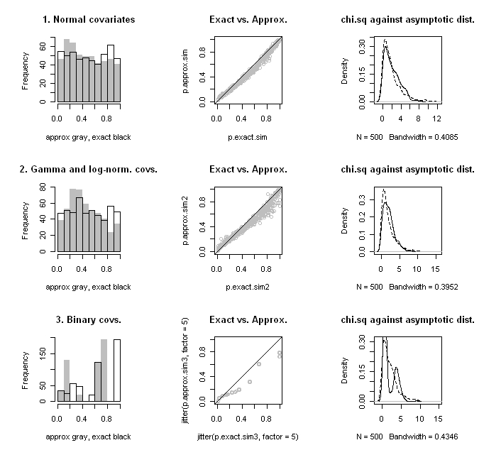
The results of the simulations are shown in the figure below. The top row is the for the normal covariates, the second row for the gamma and log-normal covariates, and the bottom row for the binary covariates. I’ve graphed the histograms for the approximate and exact p-values in the left column; we want to see a uniform distribution. In the middle column is a scatter plot of the two p-values with a reference 45-degree line; we want to see them line up on the 45-degree line. In the right column, I’ve plotted distribution of the computed $latex d^2$ statistic against the limiting $latex \chi^2_{rank[Cov(\mathbf{d})]}$ distribution; we want to see that they agree.
When the data are normal, the approximation is quite good, even with only 10 units. In the two latter cases, approximations do not fare well, as the test statistic distribution deviates substantially from what would be expected asymptotically. The rather crazy-looking patterns that we see in the binary covariates case is due to the fact that there are a small discrete number of difference in mean values possible. Presumably in large samples this would smooth out.
What we find overall though is that the approximate p-value tends to be biased toward 0.5 relative to the exact p-value. Thus, when the exact p-value is large, the approximation is conservative, but as the exact p-value gets small, the approximation becomes anti-conservative. This is most severe in the skew (gamma and log-normal) covariates case. In practice, one may have no way of knowing whether the relevant underlying covariate distribution is better approximated as normal or skew. Thus, it would seem that one would want to always use the exact test in small samples.
Code demonstrating how to compute Hansen and Bowers’s approximate test, the exact test, as well as code for the simulations and graphics is here (multivariate exact code).
Update
The general expression for $latex Cov(\mathbf{d})$ covering an unbalanced randomized design is,
$latex Cov(\mathbf{d}) = \frac{N}{M(N-M)}S(\mathbf{X})$.

