Cyrus Samii

Suppose we propose an experiment to estimate the effect of a treatment X on an outcome Y where Y is a binary 0,1 outcome. Call that effect b. If the base rate is p then the effect b is bounded to be between -p and 1-p.

Our decision problem is to decide whether treatment should be adopted. If so, the reward is b. If not the reward is 0.

Suppose if we run the experiment, we learn b, in which case we can make the optimal choice of adopting the treatment when b>0. Thus if we learn b we could ensure a payoff of max(0,b).

Suppose we collect priors on the value of b, giving rise to a prior distribution F(b). Does this prior distribution tell us about the value of running the proposed experiment to estimate b?

For example, it could be that F(b) is a spike distribution at value b=0, implying ex ante consensus that X has no effect on Y. Suppose we act on the prior, and do not implement. If the prior is exactly right, we obtain the optimal payoff of 0. If prior was actually overconfident such that b is actually negative, then again we secure the optimal payoff of 0. But if the prior was unduly pessimistic, acting on it could miss out on some gain b>0. In the absence of any other information this could be as large as 1-p. The maximum potential regret for not having run the experiment is 1-p. (Regret in this worst case is optimal 1-p minus realized 0.)

Suppose another treatment that has potential c on the same outcome, for which the base rate is still p. As before, if we ran the experiment for this treatment we could secure the optimal payoff of max(0,c). Suppose that for this second treatment however, the priors we obtain give rise to a distribution G(c) that is uniform over the interval 0 to 1-p. The prior expectation is (1-p)/2 > 0. If we acted in the basis of our prior, we would adopt the treatment., securing payoff c. If c>0, we are better off for having done so. If c<0, we would have made a mistake acting on the prior and could do as badly as -p. The maximum potential regret for not having run the experiment is p. (Regret in this worst case is optimal 0 minus realized -p.)

Under all of the assumptions above, including the different priors, the comparative value of experimenting with the first treatment versus the second depends on p.

These thoughts came to mind when listening to presentations by Brian Nosek and by Stefano Dellavigna at the BITSS conference this past week. Nosek presented a pilot project called the Lifecycle Journal, which proposes to use various existing specialized research evaluation services to quality rate facets of a study. You can obtain quality ratings for statistical power, fidelity to a pre analysis plan, and other features. He raised the intriguing possibility of obtaining a quality rating for the experiments that you are proposing to run by eliciting priors about potential effects using the Social Science Prediction Platform (SSPP). The set of quality ratings could be compiled from these separate services and then serve to establish the credibility of a study that sidesteps the need for peer review.

Later at the meeting Dellavigna presented some results from the data that SSPP has collected to date on both priors and experimental outcomes. I asked Dellavigna whether they had considered using the priors to construct ex ante metrics of the value of experiments, and he replied that they had thought about it but they hadn’t yet settled on a decision framework for doing so.

These ideas and the analysis above raise the intriguing possibility of designing a methodology for quantitatively measuring the ex ante (that is, prior to knowing any results) value of a proposed experiment. The inputs could be crowdsourced or expert-determined information about payoffs (the treatment adoption payoffs), base rate information from existing data, and then crowdsourced or expert provided priors about effect sizes (like what SSPP already does). This could put ratings about the quality of experiments on firmer ground, more like ratings about statistical power than the more taste-based judgments that you get from peer reviewers’ subjective assessments.

PS Sandy Gordon and I also presented at BITSS on a new tool called Data-NoMAD that we developed (with Patrick Su) to allow researchers to create a “digital fingerprint” of their data to allow third parties to authenticate that the data have not been manipulated. Working paper here at arXiv.

At the APSA meeting this past week I discussed a very nice working paper by Blackwell, Ma, and Opacic on testing potential causal mechanisms. Their paper enumerates the assumptions needed to justify the “intermediate outcome test”—that is, the common practice of estimating treatment effects on a mediator variable (an intermediate outcome) to test whether a proposed causal mechanism is plausible: [arxiv].

Considering the case of a binary mediator, without an assumption that the treatment effect on the intermediate outcome is monotonic, this test is not necessarily informative. You could estimate a zero average treatment effect on the mediator but the mechanism could still be active. A zero average treatment effect on the mediator could mean either that the treatment does not affect the mediator for anyone, or that the treatment has a positive effect for some and a negative effect for others, and these effects cancel out. The issue is apparent in the following expression from Blackwell et al.’s paper for the average natural indirect effect (ANIE, also known as the average causal mediation effect):

where delta(a) is the ANIE and M(a) is the potential mediator value when treatment A=a, Y(a,s) is the potential outcome when treatment A=a and mediator M=s, and then we have rho_10 and rho_01 as the probabilities that the effect of the treatment (A) on the mediator (M) is positive or negative, respectively. This expression is non parametric and a simple consequence of applying total probability. The average treatment effect on the mediator is equal to rho_10 – rho_01. You could have rho_10 = rho_01 \ne 0, in which case you would have zero average treatment effect on the mediator, but still have a potentially non-zero ANIE.

Now, the intermediate outcome test is motivated by the intuition that the mediation effect can sometimes be written as the product of the effect of the treatment on the mediator and the effect of the mediator on the outcome. From the expression above, you can see that the ANIE can be written as such a product when the conditional effects are equal, i.e., E[Y(a,1) – Y(a,0) | M(1) = 1, M(0) = 0] = E[Y(a,1) – Y(a,0) | M(1) = 0, M(0) = 1] = B, in which case the expression reduces to B*(rho_10 – rho_01). This assumption of effect homogeneity (across groups for which the effect on the mediator is positive or negative) seems pretty strong though, right?

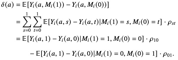
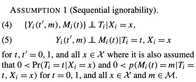
Indeed, it is strong, and, at least a conditional-on-covariates version of it is an implication of sequential ignorability as stated in, e.g., Imai et al. (2010): Personally, I had not given much thought to how the second part of the assumption (expression 5), by imposing restrictions across outcome and mediator potential outcomes, implied effect homogeneity across types defined in terms of how the treatment affects mediator values. If we consider the analogy to instrumental variables, this would be like restricting causal effects to be homogenous across compliers and defiers.

Once one appreciates this implication of sequential ignorability, other things can follow, such as using estimates of conditional effects to identify mediation effects, as in this paper by Fu: [arxiv].

I guess the question is whether we are willing to accept such restrictions on effect heterogeneity in the first place, and if not, whether we are willing to accept other restrictions on effects, such as monotonic effects of the treatment on the mediator. The answer depends on the application, but in any case these papers are important for clarifying what kinds of assumptions you need to defend.

I have a new “methodology big think” essay that argues in favor of political scientists orienting their research toward trying to address clearly-defined societal problems. Here is a link to the pdf: [pdf]

The essay is intended for a forthcoming handbook on political science methodology. I do think it makes points that would be of interest to social scientists more generally.

For some, it may seem obvious that social scientists should be working on clearly-defined societal problems. In political science, however, this is not how many people think about their research. Rather, the idea of “disinterested” or “agenda-free” pursuit of “explanation” and “puzzle solving” is very common, perhaps dominant. In my view, such an approach makes research largely an aesthetic exercise where judgments about research quality are driven by idiosyncratic tastes. That is just not the way I think about what I do, and frankly, if such a “disinterested” approach were to define our discipline, I’d have a hard time explaining why anyone should devote serious resources to it. There are much more compelling ways to meditate on the exercise of power and the human condition than “disinterested” regression studies in a political science journal.

The essay argues that taking a “problem-solving” mindset can help to organize one’s thinking about methodological questions. I propose that a problem-solving research program operates through three steps: (1) problem definition and description, (2) primarily observational examination of mechanisms that perpetuate the problem, and (3) primarily experimental studies to test intervention strategies to mitigate the problem. Social scientists should develop skills to operate through each of these stages, although some specialization in one of the phases makes perfect sense. Social science journals should devote nearly equal space to each of these types of research.

I have organized my teaching, advising, and assessments of research on the basis of this mindset. I think it is very powerful, and it helps me to address questions of priority in a systematic way. I think that students find it clarifying too.

My thinking is strongly influenced by recent contributions by Duflo ([link]) in economics and Moynihan ([link]) in public administration. I highly recommend these.

I would love to know what you think.

Greenland and Pearl (2017) [link] offer a fully graphical strategy based on “graph moralization” as a way to figure out conditioning strategies for causal identification problems using directed acyclic graphs (DAGs). I don’t see this presented as often as it should, given how powerful it is and, also, how incredibly easy and intuitive it is. The graph moralization approach is how I teach conditioning strategies using DAGs (e.g., [link]).

The way I teach it is like this:

1. Start with the DAG that represents the actual data-generating process (DGP).
2. Next define a “target intervention graph” that represents, in DAG form, an ideal experimental DGP for the causal effects that you want to identify.
3. Apply the graph moralization rules per Greenland and Pearl to check the implications of conditioning on different variables in the DAG for the actual DGP.
4. You have identified a sufficient conditioning set when you have gotten the actual DGP DAG to look like the target intervention graph through conditioning and moralization. Note that for any given problem, there may be more than one conditioning set that is sufficient.

The graph moralization rules are as follows, quoting Greenland and Pearl:

Conditioning on a variable C in a DAG can be represented by creating a new graph from the original graph to represent constraints on relations within levels (strata) of C implied by the constraints imposed by the original graph. This conditional graph can be found by the following sequence of operations, sometimes called graphical moralization.

1. If C is a collider, join (marry) all pairs of parents of C by undirected arcs.
2. Similarly, if A is an ancestor of C and a collider, join all pairs of parents of A by undirected arcs.
3. Erase C and all arcs connecting C to other variables.

(Greenland and Pearl, 2017, pp. 3-4)

Recently, @analisereal posed an identification conditioning problem:

In the spirit of the Crash Course, here’s another puzzle, brought to you by Ema Perkovic. Suppose you want to identify the total effect of a joint intervention of X1 and X2 on Y. Which variables should you include in you regression equation? U is unobserved. Quiz in next tweet. https://t.co/XFSYgozc3f pic.twitter.com/2Td7TeqXMl

— Análise Real (@analisereal) April 10, 2022

We can apply the recipe outlined above. The DAG in the tweet represents the actual DGP. The target intervention graph needs to represent “a joint intervention of X1 and X2 on Y.” This would be as follows:

To see what happens when we condition on the available controls, we would apply the graph moralization rules. Conditioning on Z2 would require that we apply rules 1 and 3, yielding: So we are not quite there with respect to our target graph. That said, the graph that results here is interesting, because it does capture a DGP that characterizes two conditionally independent effects of X1 and X2 on Y, and thus it does capture the effects of a joint intervention of X1 and X2 on Y in circumstances in which Z2 is held fixed. It’s just that the mediation pathway between X1 and Y is obscured relative to our target graph.

Conditioning only on Z1 (and not Z2) would require that we apply rule 3, yielding: Here, we have a DGP that is clean for the effect of X1 on Y, but the effect of X2 on Y is confounded by a backdoor path.

Conditioning on both Z1 and Z2 results in the following: The variable U is exogenous, and so we can remove it from the graph. This gets us to our target intervention graph, and represents a solution to the problem.

Now, when effects are heterogeneous with respect to conditioning variables, then we should have a way to remind ourselves that we need to marginalize conditional effect estimates over values of the conditioning variables. This would be necessary in order to get to a population-level estimate of the effects on the target intervention graph. The way I like to do it is to write the conditioning arguments next to the conditional graph, like this: Writing out “Z1=z1, Z2=z2” by the graph makes it clear that these are conditional relationships on the actual DGP, and that marginalization (with respect to z1 and z2) would be needed to get from this to the effects that target intervention graph represents in the population.

I am putting these notes here to remind me of steps and also in case others are curious about doing something similar.

Suppose we want to situate a scholar in their field, for example as part of a tenure review case. One way to do that is to look at the scholar’s papers and see who they are citing:

1. Go to their Google scholar profile and pull up their papers. Choose some of their most cited papers (reflecting how others see the scholar’s contributions) and some of their most recent papers (reflecting their current thinking).

2. Construct the network of people that the scholar references in their most prominent work.

A low-tech way to do this is to copy/paste bibliographies from the papers into https://anystyle.io/ to put the bibliographies into machine readable format (e.g., bibtex). I like to tag the entries from each paper’s bibliography by the date of the paper’s publication (e.g., by adding a custom field to the bibtex file) so that I can sort and see how the scholar’s reference base has changed over time. Compile the different bibliographies into a library in a reference manager. If you keep duplicate entries you get a sense of the scholar’s key points of reference.

A higher-tech way to do this is to use the Connected Papers app. You can look at the graph to find well-cited work that the scholar tends to reference.

UPDATE (12/14/23): The “InfluenceMap” project allows for creating an influence diagram (people that the scholar draws up, and then people who cite the scholar): [link]

1. Pare down the list to seminal contributions. E.g., keep only entries from relevant general interest and field journals that are highly cited.

Now some analyses:

First, who appears most often in the library? What does the work of these primary referents represent in the literature and how does the current scholar’s work relate?

Second, whose work is being referenced at different times over the course of the scholar’s career (I do this using the custom field described above)? What does this say about how the scholar’s work has evolved alongside the reference literature?

As far as I know, the steps above are not as well-automated as methods to see who else is citing the scholar’s work (there are numerous tools to do that, like the “scholar” package in R). Would love to see someone do it (and welcome any suggestions below).