Greenland and Pearl (2017) [link] offer a fully graphical strategy based on “graph moralization” as a way to figure out conditioning strategies for causal identification problems using directed acyclic graphs (DAGs). I don’t see this presented as often as it should, given how powerful it is and, also, how incredibly easy and intuitive it is. The graph moralization approach is how I teach conditioning strategies using DAGs (e.g., [link]).
The way I teach it is like this:
- Start with the DAG that represents the actual data-generating process (DGP).
- Next define a “target intervention graph” that represents, in DAG form, an ideal experimental DGP for the causal effects that you want to identify.
- Apply the graph moralization rules per Greenland and Pearl to check the implications of conditioning on different variables in the DAG for the actual DGP.
- You have identified a sufficient conditioning set when you have gotten the actual DGP DAG to look like the target intervention graph through conditioning and moralization. Note that for any given problem, there may be more than one conditioning set that is sufficient.
The graph moralization rules are as follows, quoting Greenland and Pearl:
Conditioning on a variable C in a DAG can be represented by creating a new graph from the original graph to represent constraints on relations within levels (strata) of C implied by the constraints imposed by the original graph. This conditional graph can be found by the following sequence of operations, sometimes called graphical moralization.
- If C is a collider, join (marry) all pairs of parents of C by undirected arcs.
- Similarly, if A is an ancestor of C and a collider, join all pairs of parents of A by undirected arcs.
- Erase C and all arcs connecting C to other variables.
(Greenland and Pearl, 2017, pp. 3-4)
Recently, @analisereal posed an identification conditioning problem:
In the spirit of the Crash Course, here’s another puzzle, brought to you by Ema Perkovic. Suppose you want to identify the total effect of a joint intervention of X1 and X2 on Y. Which variables should you include in you regression equation? U is unobserved. Quiz in next tweet. https://t.co/XFSYgozc3f pic.twitter.com/2Td7TeqXMl
— Análise Real (@analisereal) April 10, 2022
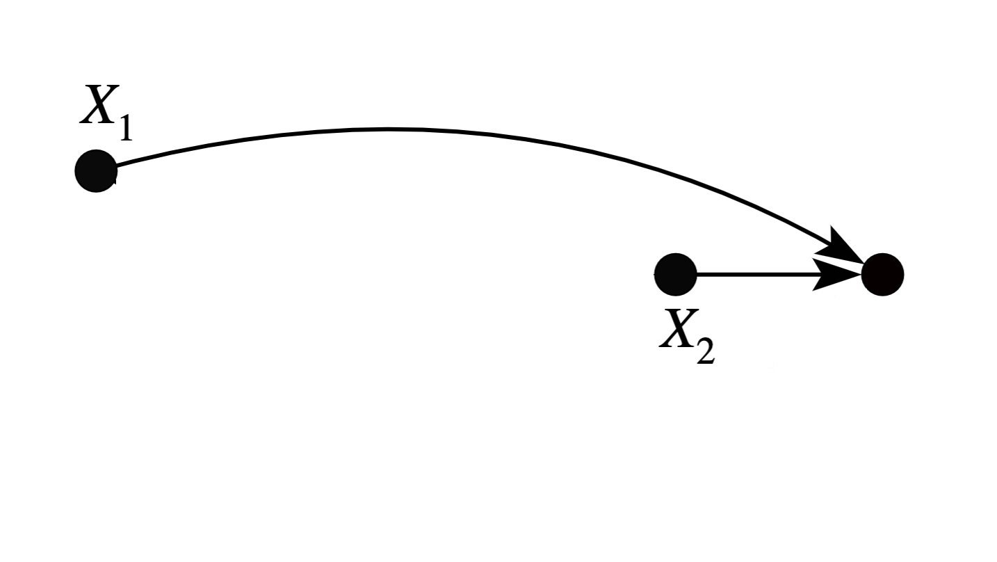
We can apply the recipe outlined above. The DAG in the tweet represents the actual DGP. The target intervention graph needs to represent “a joint intervention of X1 and X2 on Y.” This would be as follows:
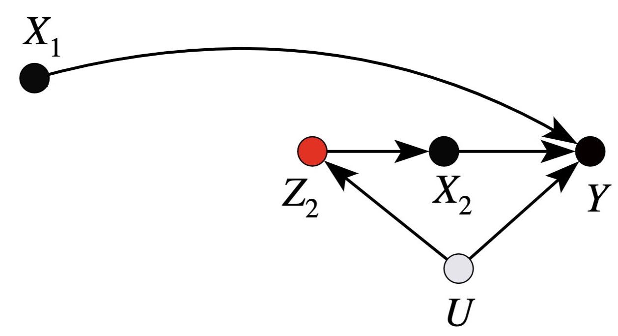
To see what happens when we condition on the available controls, we would apply the graph moralization rules. Conditioning on Z2 would require that we apply rules 1 and 3, yielding:
So we are not quite there with respect to our target graph. That said, the graph that results here is interesting, because it does capture a DGP that characterizes two conditionally independent effects of X1 and X2 on Y, and thus it does capture the effects of a joint intervention of X1 and X2 on Y in circumstances in which Z2 is held fixed. It’s just that the mediation pathway between X1 and Y is obscured relative to our target graph.
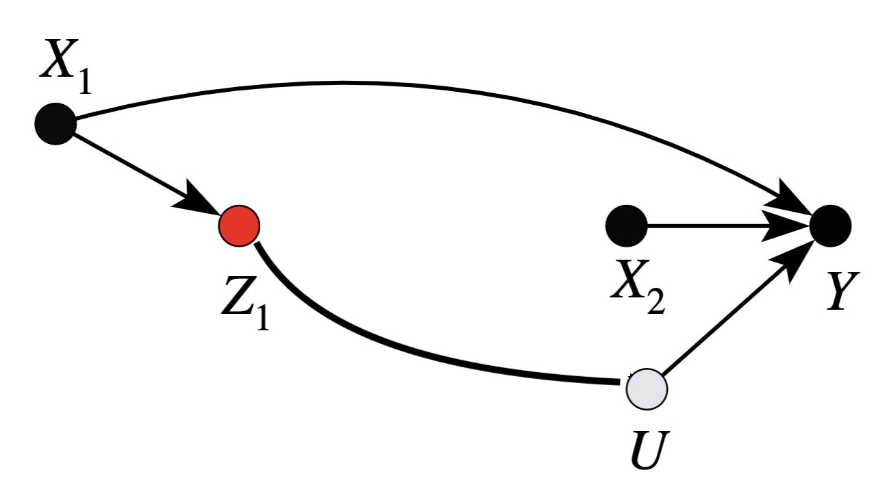
Conditioning only on Z1 (and not Z2) would require that we apply rule 3, yielding:
Here, we have a DGP that is clean for the effect of X1 on Y, but the effect of X2 on Y is confounded by a backdoor path.
Conditioning on both Z1 and Z2 results in the following:
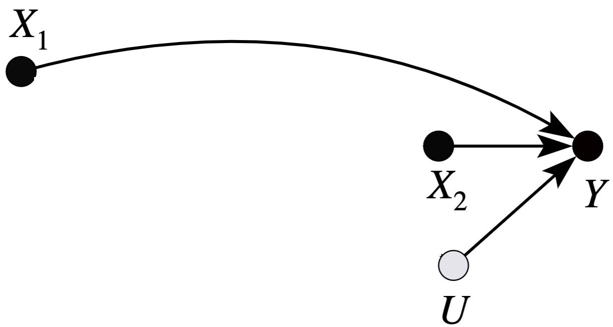
The variable U is exogenous, and so we can remove it from the graph. This gets us to our target intervention graph, and represents a solution to the problem.
Now, when effects are heterogeneous with respect to conditioning variables, then we should have a way to remind ourselves that we need to marginalize conditional effect estimates over values of the conditioning variables. This would be necessary in order to get to a population-level estimate of the effects on the target intervention graph. The way I like to do it is to write the conditioning arguments next to the conditional graph, like this:
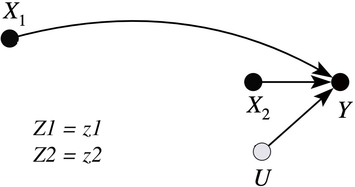
Writing out “Z1=z1, Z2=z2” by the graph makes it clear that these are conditional relationships on the actual DGP, and that marginalization (with respect to z1 and z2) would be needed to get from this to the effects that target intervention graph represents in the population.