Cyrus Samii

From the Microcon/HICN email list:

The Households in Conflict Network (HiCN) is seeking a Short-Term Consultant to prepare a project proposal on the social and political transformation in the Arab world. The research project will focus on determinants, forms and effects of individual participation in the recent protests across the region. We are looking for a consultant, available on short notice, to write a complete research proposal in collaboration with project’s international partners.

Successful candidates should have a master’s or doctoral degree in economics, political science, sociology or development studies. Excellent English, proven writing skills, grant writing experience, and the ability to work independently under tight deadlines are essential prerequisites. Interest in the MENA region, and a working knowledge of Arabic would be an advantage.
Candidates should be available to work full-time on this project for 4 months from October 2011 till 5 February 2012. The remuneration is competitive, and the consultant must be available to work in Berlin. Applications from abroad are encouraged, but the successful candidate must be willing to relocate to Berlin for the period of the project.

If you are interested, please send a detailed CV, letter of motivation, reference letter (if available), and one recent writing sample in English by email to Mira Purska (mpurska [at] diw.de). The deadline for applications is 26 September 2011. Only shortlisted candidates will be contacted for an interview.

United States and France [are] two countries…generally viewed as polar opposites as far as the political legitimacy and legal validity of race-based classifications are concerned. Based on an in-depth study of recent programs designed to increase the “diversity” of the student body in selective institutions of higher education, I will argue that French and U.S. policies are currently converging around the instrument of indirect (and often implicit) affirmative action.

[W]hat might be the causal mechanisms involved [in this convergence]? There is not even a shred of evidence that the policy convergence…is the result of a diffusion process. [Rather]…the rise of indirect affirmative action is linked to the widespread endorsement of the quintessentially political metagoal…“to integrate the national community by rubbing out in the [public’s] consciousness (…) a perception of racial difference”…that is, to reduce the salience of racial boundaries and eventually “eliminate race” as a principle of social organization. Because policies unavoidably have an expressive as well as an instrumental dimension, the very existence of an allocative scheme taking account of race in a transparent way is likely to jeopardize the “deracialization” that one is trying to bring about in the long run. So long as the criterion of race is seen to operate at the preliminary stage of identifying the participants in the interaction process, it remains unlikely that racial decategorization will occur.

From Daniel Sabbagh’s paper in the current issue of World Politics (gated link). For France, his primary evidence comes from recent experimentation with diversity-based admissions at Sciences Po. For the US, his evidence comes from a variety of examples where explicit race-based provisions, despite their constitutional admissability, have been eschewed in favor of measures that seem intentionally to obfuscate de facto race-based preferential treatment.

Affirmative action policies are a research interest of mine, and Sabbagh has done interesting work, though his focus is mostly on wealthy countries whereas mine is more on lower income and primarily post-conflict countries. Worth a look as well is his syllabus on comparing affirmative action policies (link).

For NYU and NYC-area graduate students, Joel Middleton and I are planning a year-long sequence that will train graduate students to design and analyze surveys and field experiments. Here’s the announcement:

=====================

The PRIISM Center would like to bring to your attention the following complementary course offering that involve NYU’s Steinhardt School and its Graduate School of Arts & Sciences (GSAS). More information, including dates/times of instruction can be found here: http://steinhardt.nyu.edu/humsocsci/interdepartmental/courses or through links to the sponsoring departments at this site: http://steinhardt.nyu.edu/priism/courses

Series on Sampling, Design, and Inference:

This year-long series will cover both introductory and advanced topics in the design and analysis of sample surveys and social experiments. The series will consist of a Fall course titled, “Sampling, Design, and Inference I: Survey Research Methods,” taught through the Steinhardt School, and a Spring course titled, “Sampling, Design, and Inference II: Quantitative Field Methods,” taught through the GSAS Politics Department. The Fall 2011 course will be an introductory and hands-on overview for graduate students who plan to carry out or analyze sample surveys. The Spring 2012 course will provide advanced training in sampling and will extend these techniques to experimental design and analysis. A brief description follows.

RESCH-GE 2139 Sampling and Inference I: Survey Research Methods (3 points)
Instructor: Joel Middleton (Steinhardt School), FALL 2011

This course will be based on an existing Survey Research Methods course that has been offered through Steinhardt in recent years, previously taught by Jack Buckley. Undergraduate-level introductory statistics is required but no previous experience with survey research is presumed. This course intends to train graduate students in the following: total survey error; creation and pre-testing of survey instruments; basic principles of sampling, power, measurement, and design-based inference; analysis of data from sample surveys using design-based and model-based analytical techniques. The texts for this course will be at the level of Groves et al., Survey Methodology, Wiley, 2004, with selected readings from Lohr, Sampling: Design and Analysis, Duxbury, 1999.

POL-GA 3200 Sampling and Inference II: Quantitative Field Methods (4 points)
Instructor: Cyrus Samii (GSAS/Politics), SPRING 2012

This is a more advanced graduate course for those who wish to go further than what is provided in the Survey Research Methods course and to become expert in sampling and field experiment methodology. Prerequisites will be introductory graduate-level statistics. The Survey Research Methods course (or equivalent) is recommended though not required. This course will cover: foundations of sample-theoretic and randomization-based estimation and testing; optimal design of samples and experiments via stratification and adaptive designs; non-standard design problems, including network samples and other forms of “indirect” sampling and randomization; estimation and testing under clustering, interference, non-compliance, and other non-standard scenarios; examination of state of the art sampling, field experiment, and survey experiment studies. The texts for this course will be at the level of Sarndal et al., Model Assisted Survey Sampling, Springer, 1992, and Imbens and Rubin, Causal Inference in Statistics, Cambridge, forthcoming.

=====================

While Joel and I will teach these two classes separately, we are each planning guest appearances in each others’ classes on special topics. Hope to see you there.

As with all sorts of data analysis scenarios, when you are carrying out a regression discontinuity (RD) study, you might have some missing data. For example, suppose you are using the (now, classic) Lee (2008) research design to estimate the effects of being elected to political office (ungated link; but note critiques of this design as discussed here: link). In this design, we exploit the fact that in plurality winner-take-all elections, there is an “as if” random aspect to the outcomes of elections that have very close margins of victory. E.g., a two-candidate race in which the winner got 50.001% of the vote and the loser got 49.999% is one in which one could imagine the outcome having gone the other way. Thus, using margin of victory as a forcing variable sets you up for a nice RD design. But, the rub is that you need data on both the winners and the losers in order to track the effects of winning versus losing. Unfortunately, it may be the case that data on the losers is hard to come by. They may drop out of the public eye, and so you will have a selected set of losers that you are able to observe. That is, you have missing outcome data on losers.

In a working paper in which I review semi-parametric methods for handling missing data, I discuss how inverse probability weighting (IPW), imputation, and their combination via “augmented” inverse probability weighting (AIPW) might be well suited to the task to dealing with missing data for RD designs (link to working paper). The problem with these methods, though, is that they rely on an “ignorability” assumption: that is, for the cases whose outcomes are missing, you nonetheless have enough other information on them to be able either (i) to predict well whether they are missing or (ii) to predict well what their outcomes would have been had they been observed. Ignorability is a strong and untestable assumption. Thus, in the paper I discuss very briefly the idea of doing sensitivity analysis to examine violations of ignorability.

I am currently re-working that paper, and in doing so working out how exactly such a sensitivity analysis ought to be carried out. As a useful prompt, I received an email recently asking precisely what one might do to study sensitivity to missing data in the RD scenario. My proposal was that one could do a couple of things. First, one could compute bounds based on imputing extreme values for the missing outcomes, and seeing what that suggests. This would be along the lines of a Manski-type “partial identification” approach to studying sensitivity to missing data (see Ch. 2 in this book: link). Second, one could do an IPW adjusted analysis (keeping to the side imputation and AIPW for the moment), and see how your results change. Third, one could do a sensitivity analysis for the IPW analysis. A sensitivity analysis that I imagine is to take the complete cases and residualize their outcome variable values relative to the forcing variable and any other covariates used to predict the missingness weights. Then, scale these residuals relative to the strongest predictor of missingness (determined, for example, using a standardized regression analysis). And finally, examine the consequences of increasing the influence of these scaled residuals in predicting missingness. Then, you would have a way to examine sensitivity to ignorability in a manner that is scaled to the strongest predictor and its influence.

These suggestions were a bit off the cuff, although they made intuitive sense. Nonetheless, I wanted to check myself. So I did a toy simulation. The findings were surprising.

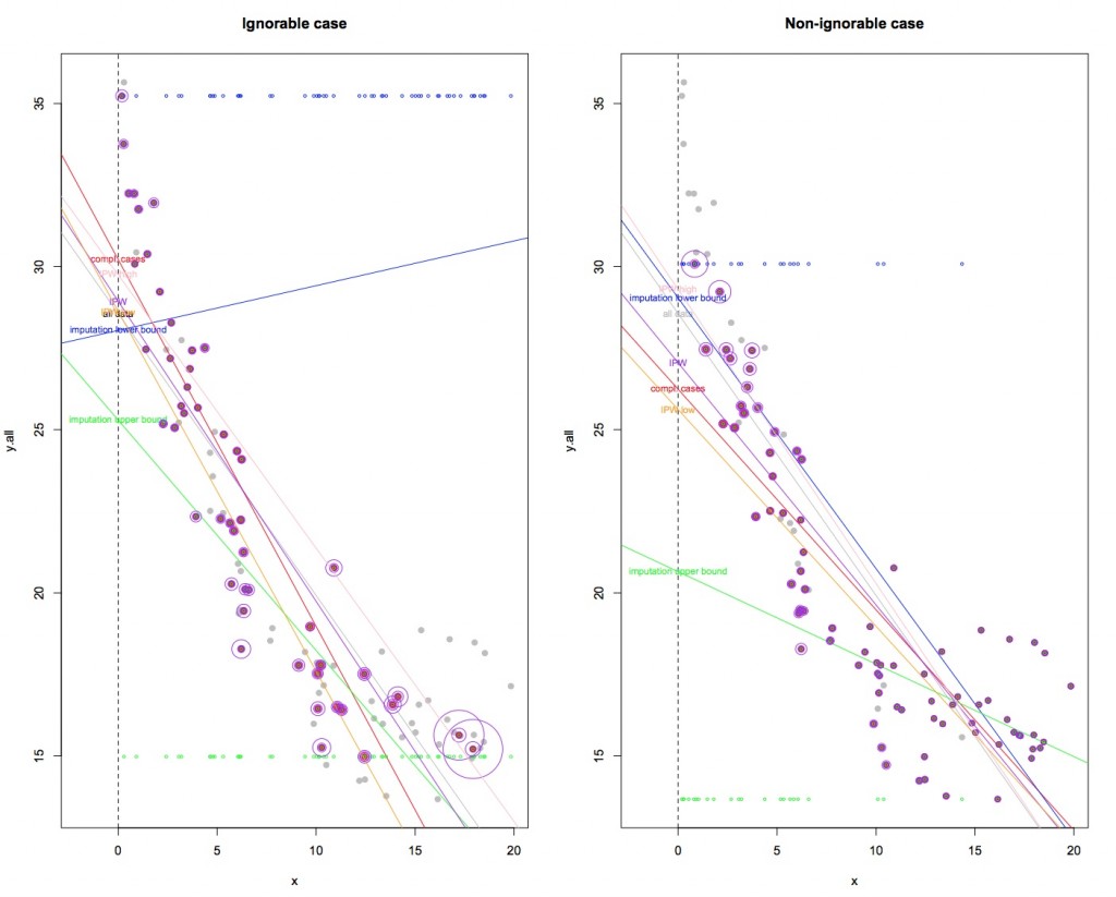
The R code for the toy simulation is here: R code.[1] The code contains two examples of trying to predict an intercept value using a local linear approximation to a non-linear relationship. This is one side of what one is trying to do in a standard RD analysis. In one example, ignorability holds, and in the other it does not. Ideally, what I would like you to do is to run that code line by line in R and look at the graphical output that shows the result of each approach to addressing the missing data problem. The steps include, first computing a benchmark prediction that would obtain were there no missingness (“all data” scenario). Then, we look at predictions resulting from,

(1) doing nothing — aka, complete case analysis (“compl. cases” scenario);

(2) imputing extrema (“imputation lower bound” and “imputation upper bound”, where lower and upper are referring to whether min or max values are imputed);

(3) IPW adjustment (“IPW”), and then

(4) an IPW sensitivity analysis along the lines discussed above (“IPW low” and “IPW high”).

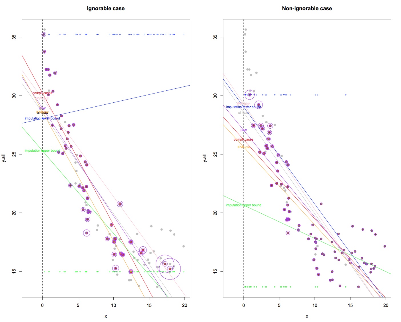
For those who can’t run the code, here is a (very crowded) PDF that graphs color-coded results for the two examples: PDF. You will have to zoom in to make sense of it. It shows where all the predictions landed. We want to be in the neighborhood of the intercept prediction labeled “all data”.

Here are the basic conclusions from this toy simulation. First, and most importantly, the bounds from imputing extrema don’t necessarily cover what you would get if you had all the data! This occurred in the ignorable case. This was surprising to me and it’s worth considering more deeply. The problem is due to the fact that one is trying to predict an intercept here, and so imputing high or low values for the missing data does not necessarily imply that the resulting intercept estimate will cover what you would get with the full data. It seems that the linear approximation to the non-linear relationship is compounding the problem, but that is a conjecture that needs to be assessed analytically. I found this quite interesting, and it suggests that what we know about sensitivity analysis for simple difference in means types estimation does not necessarily travel to the RD world.

Second, the IPW sensitivity analysis is pretty straightforward, and works as expected. However, it requires that you choose—more or less, out of thin air—what defines an “extreme” violation of ignorability. Also, the IPW sensitivity analysis still leaves you with a fairly tight range of possible outcomes. This is not necessarily a good thing, because the tightness might imply that there are still some assumptions that aren’t being subjected to enough scrutiny. So I think this is a promising approach, but probably needs a lot of consideration and justification when used in practice.

Third, in these examples, IPW always removed at least some of the bias, although there are cases where this may not happen (see p. 21 of my paper linked above for an example).

So there are some interesting wrinkles here, the most important being that Manski type approaches may not travel well to the RD scenario. I need to check to be sure I’m not doing something wrong, but assuming I didn’t that’s an important take-away.

[1] Okay, the code is pretty rough in that lots of things are repeated that should be routinized into functions, but you know what? I never claimed to be a computer programmer. Just someone who knows enough to get what I need!

1. A post from last week by Jenny Aker at the Savings Revolution blog (link) proposes strategies for rigorous impact assessment when full randomization is not possible. Her third suggestion is a friendly way of saying that regression discontinuity (RD) designs should be used more, not only in analyzing existing interventions, but in designing new ones. If we can use quantifiable indices to determine who qualifies to receive program benefits, and if the indices are used faithfully in actually determining who gets benefits, then we can use the indices to carry out an RD analysis. This should be appealing to practitioners because it provides a transparent and relatively incorruptible method for beneficiary selection and it is sensitive to concerns that those most in need be most eligible for assistance, while minimally compromising our ability to estimate program impacts. As methodologists, I think we need to do more to sell this approach in cases where full randomization is not feasible.

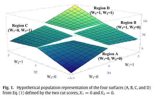
2. A relatively new paper by Papay et al. in Journal of Econometrics (gated link) demonstrates ways to generalize RD analysis to multiple assignment variables and cutoffs in multiple dimensions. The killer graph from the paper is shown above. In this case, you have treatment assignment based on cutoffs on two variables, labeled as X1 and X2 on the graph (the vertical axis is the outcome variable). Cutoffs in two dimensions create four treatment regions, A, B, C, and D. The analysis proceeds by using a regression to model the response surface in each region. Then, you can obtain predicted values along each of the discontinuity edges. These predictions can be subtracted from each other and aggregated to produce various types of average treatment effects. All of this can happen more or less automatically with a single regression specification, although one should take care to understand the manner in which such a regression “averages” the various available treatment effects (I believe that it produces a covariance-weighted average, rather than a sample weighted average, along the lines of what Angrist and Pischke discuss in Mostly Harmless…).

3. A colleague and I were discussing tests for the identifying assumptions for RD. It seems that there have been some calls to test for “balance” in covariates around cutpoints to assess whether identifying assumptions are met for RD. The idea of these tests is that in the neighborhood of the cutpoint, covariate distributions should be equal. Balance is thus tested using the permutation distribution under this null hypothesis. To me, this sounds like one is imposing more assumptions than necessary for an RD design. RD requires smoothness in covariates, not balance. The “R” in RD is there for a reason. If balance were a necessity, we should just call it “D”! Covariate means might differ on either side of the cutpoint within arbitrarily small windows, without there being a violation of the smoothness condition. In this case, a balance test would lead one to conclude that identifying conditions are not met when in fact they are (that is, the test would be trigger happy on the type II error rate). The direct test for smoothness is a “placebo” regression of the covariate, where you estimate the existence of a discontinuity (refer to Imbens and Lemieux, gated link). I suppose one could construct a permutation test that also looks for smoothness/discontinuities, but the balance tests on adjusted covariates strikes me as erroneous.