1. A post from last week by Jenny Aker at the Savings Revolution blog (link) proposes strategies for rigorous impact assessment when full randomization is not possible. Her third suggestion is a friendly way of saying that regression discontinuity (RD) designs should be used more, not only in analyzing existing interventions, but in designing new ones. If we can use quantifiable indices to determine who qualifies to receive program benefits, and if the indices are used faithfully in actually determining who gets benefits, then we can use the indices to carry out an RD analysis. This should be appealing to practitioners because it provides a transparent and relatively incorruptible method for beneficiary selection and it is sensitive to concerns that those most in need be most eligible for assistance, while minimally compromising our ability to estimate program impacts. As methodologists, I think we need to do more to sell this approach in cases where full randomization is not feasible.
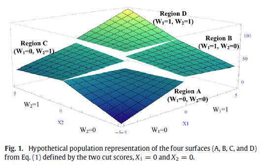
2. A relatively new paper by Papay et al. in Journal of Econometrics (gated link) demonstrates ways to generalize RD analysis to multiple assignment variables and cutoffs in multiple dimensions. The killer graph from the paper is shown above. In this case, you have treatment assignment based on cutoffs on two variables, labeled as X1 and X2 on the graph (the vertical axis is the outcome variable). Cutoffs in two dimensions create four treatment regions, A, B, C, and D. The analysis proceeds by using a regression to model the response surface in each region. Then, you can obtain predicted values along each of the discontinuity edges. These predictions can be subtracted from each other and aggregated to produce various types of average treatment effects. All of this can happen more or less automatically with a single regression specification, although one should take care to understand the manner in which such a regression “averages” the various available treatment effects (I believe that it produces a covariance-weighted average, rather than a sample weighted average, along the lines of what Angrist and Pischke discuss in Mostly Harmless…).
3. A colleague and I were discussing tests for the identifying assumptions for RD. It seems that there have been some calls to test for “balance” in covariates around cutpoints to assess whether identifying assumptions are met for RD. The idea of these tests is that in the neighborhood of the cutpoint, covariate distributions should be equal. Balance is thus tested using the permutation distribution under this null hypothesis. To me, this sounds like one is imposing more assumptions than necessary for an RD design. RD requires smoothness in covariates, not balance. The “R” in RD is there for a reason. If balance were a necessity, we should just call it “D”! Covariate means might differ on either side of the cutpoint within arbitrarily small windows, without there being a violation of the smoothness condition. In this case, a balance test would lead one to conclude that identifying conditions are not met when in fact they are (that is, the test would be trigger happy on the type II error rate). The direct test for smoothness is a “placebo” regression of the covariate, where you estimate the existence of a discontinuity (refer to Imbens and Lemieux, gated link). I suppose one could construct a permutation test that also looks for smoothness/discontinuities, but the balance tests on adjusted covariates strikes me as erroneous.

